1 Introduction and Theoretical Background
For rheological measurements - and in general for any spectroscopic technique - there is a clear need for the most sensitive detection possible. The maximum sensitivity limits the possible accuracy of the observed phenomena and consequently the minimum detectable changes. Most spectroscopic techniques push these limits further back via both soft and hardware developments. Especially for spectroscopic techniques with inherently weak signals (e.g., NMR-spectroscopy) great effort has been put into the compensation of this lack of sensitivity. Generally applied attempts to overcome this problem are to develop more sensitive detection devices, shielding of spurious signals, and finally smarter data acquisition and appropriate data processing software. The goal of this article is to illustrate the potential of a data acquisition and handling routine - which has become available in recent years - of the source of raw rheological data, the torque sensor.
Within this article we would like to define sensitivity as the ratio of any detected signal S to the noise N. The noise N will result in the uncertainty of the measured quantity. Noise itself can originate from several sources and can be separated into random noise and systematic noise. The ratio between S and N is also called the relative accuracy and is also expressed by S/N. It should be noted that there is an important distinction between sensitivity and selectivity and that these two terms are frequently confused. Sensitivity quantifies the intensity of a signal towards the related noise, whereas selectivity quantifies the relative separation from one signal to an adjacent signal, e.g., the separation of two peaks in NMR or IR-spectra. Due to the fact that for rheological measurements almost always only a single frequency is applied, selectivity is only of minor importance. To increase the S/N-ratio it is generally possible to take the average over n measurements or cycles where the sensitivity grows, in case of random noise, as the square root of the measured transients, S/N ∞ n1/2 (Skoog and Leary 1992). The averaging technique therefore requires longer measurement times. Systematic noise does not follow this simple relation. In the worst case scenario averaging techniques do not improve the S/N ratio at all.
For rheological measurements under oscillatory conditions the data acquisition is - to our knowledge - so far performed by lock-in amplifiers or by calculating the Fourier transform (FT) spectra at the excitation frequency using the time response of the torque sensor. If the assumption of linear response is sufficient there is no need to calculate the whole frequency spectra. Only a single data point of the response function within the FT- spectrum at exactly the excitation frequencyω1/2π needs to be considered. The numerical value of the absolute amplitude and relative phase lag with respect to the oscillatory excitation can directly be converted into G' and G".
We would like to demonstrate in this article the possibility of increasing the force, respective torque sensitivity using a straightforward data acquisition and processing technique enabled by modern analog to digital converter (ADC) cards.
The basic idea is to acquire the oscillatory shear time data at the highest possible acquisition rate as allowed by a modern ADC, thereby exceeding by far the required minimum of three data points per cycle that would define frequency, amplitude, and phase of the response signal; the raw data is "oversampled". The sampling rate may exceed 50 kHz with this method, even for a simple oscillatory shear experiment where, e.g., a ω1/2π= 1 Hz shear frequency is applied. In a second step the raw time data is truncated "on the fly" by means of a so-called "boxcar" average over, e.g., several hundreds or thousands of raw data points (Skoog and Leary 1992). To take a boxcar average one simply calculates the average over a fixed number of data points between t and t +Δt that results in a single data point at t + 0.5△t. Each of these new values has an inherently lower relative noise level due to the applied averaging procedure. The application of the boxcar average to the raw time data results in a new time domain data set with a strongly reduced number of data points and reduced random noise for each new data point. Up to a few years ago, however, such oversampling would produce gigantic data sets since averaging could only be applied after finishing the measurement. To give an example, sampling 50 cycles with 0.1 Hz shear excitation at a sampling rate of 10 kHz would result in 5 x 10⁶ time data points.
To illustrate the described boxcar procedure for the unfamiliar reader we consider the following example (see also Fig. 1). Let us assume that the shear excitation frequency is ω1/2π= 1 Hz and originally ten data points (of typically 10μs duration) every tdw= 100ms are acquired from the force transducer over one shear cycle (line A in Fig. 1). If oversampling at a 1 kHz rate is used for a single cycle, then 1000 data points are acquired first (line B in Fig. 1) and subsequently reduced to 10 data points by truncation over 100 data points, each now spaced by 100 ms (line C in Fig. 1). The averaging of 100 data points per boxcar interval reduces the random (but of course not the systematic!) noise within this interval by a factor of S/N∝1001/2= 10, which we consider a significant sensitivity improvement. After this first pre- averaging step the data is analyzed in the usual way. The basic idea of this method is displayed in Fig. 1 for an artificial data set where noise with a standard deviation of σ=0.5 was added to a sinusoidal function with unit amplitude. A sinusoidal function is also shown as a bold trace in line B.
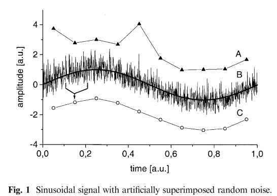
The standard deviation of the noise σ=0.5 is chosen to be half the amplitude A= 1 of the sinusoidal signal. In trace A, typical data points every 0.1 time steps are displayed. In trace A, hardly a harmonic signal is visible. Trace B shows the signal if a 100 times faster data acquisition is applied, also the pure sinusoidal signal is shown in bold for convenience. The boxcar average over 100 data points results in trace C. Clearly the noise is strongly reduced in C, the sinusoidal shape is recovered, while at the same time amplitude and phase of the oscillation are preserved.
It should be realized that most ADCs continuously measure an electric signal. For a typical commercial 100- kHz ADC each data point is averaged over 10μs. If lower acquisition rates are applied the ADC simply ignores all other time data and only at the assigned sampling interval a window of typically 10μs is opened and serves as information source. This way a sampling rate of 10 Hz ignores 99.9% of the raw signal. The 99.9% ignored raw data are basically our source of information that we would like to incorporate into the analysis. With this "Gedankenexperiment" it is also clear that the relative improvement via this method should be more efficient for lower excitation frequencies where a higher percentage of the raw data is ignored.
Until recently most ADC-cards had a fixed on-board memory of 64kB with 12-16 bit resolution. If the buffer is filled first and then the memory is transferred to the memory of the PC, during this time no data can be acquired. This transfer may take some milliseconds or longer, depending on the hard and software. Consequently one will have an undefined time gap between two data sets, which can only be corrected for if an accurate hardware-time is known.
For rheological measurements this normally means that the 64 k B time data points are sampled equidistant over the shear cycle after which they are transferred and Fourier transformed. Measuring longer or over several cycles does not increase the S/N, unless several subsequent traces are averaged.
However, modern PCI-ADC cards with bus mastering can transfer data from its data buffer (within the PC memory) to the computer where boxcar data averaging takes place, while the PCI-ADC card simultaneously samples the signal. As a result, measuring for a longer time is useful since it directly increases the number of acquired data points. This method reduces the output data set with a significant factor (typically 102- 105; a welcome reduction for the Discrete FT). The new time data set is processed afterwards in the usual way to extract the rheological parameters, e.g., torque, G', and G".
The theoretical limit of oversampling is given by the non-random noise and also by the maximum sampling rate. In the limit of fast sampling it seems even more convenient to integrate the signal. Exactly this is done routinely, e.g., in NM R-spectroscopy a narrow band width filter is applied to the raw signal before it is passed to the ADC (Homans 1989). A narrow band width filter allows only a certain frequency band v0土Δv to pass and is analogous to an integration over a time interval △t ∞ 1/Δv. This statement can be proven by a simple Fourier transform argument (Ramirez 1985; Bracewell 1986).
A further and perhaps also important advantage of oversampling is related to the artificially increased dynamical range of the ADC, see also (Derome 1993; Wilhelm et al. 1999). A typical 16-bit ADC can discriminate 216-1 = 65,535 discreet steps with respect to the signal intensity. This would be related to a dynamical range of 10 X log(Imax/Imin)= 10 x log(65,535)= 48 dB simply due to the ADC's discretization steps. Therefore, this dynamical range severely limits the minimum detectable torque, even if the appropriate pre-amplification is used. The boxcar average of k data points increases the dynamical range by 10 X log(k) because the averaging procedure generates a finer intensity discrimination. Consequently, the averaging of 1000 time data points results in an artificially enhanced dynamical range of48dB+30dB=78dB.
Although we routinely apply the above described procedure under non-linear, large amplitude oscillatory shear (LAOS) conditions, the enhanced sensitivity of the force transducer is of course also applicable in the linear regime. Information with respect to the mathematics and the application of FT to non-linear rheology can be found in Wilhelm et al. (1999) and references therein.
It is worth mentioning that the success of this approach is based on the assumption that the lower sensitivity limit of the force transducer is determined by random noise, at least to a significant degree. If the lower limit would only be caused by systematic errors this method could not result in significant S/N improvements.
2 Experimental
Data were obtained using a Rheometric (USA, NJ Piscataway) Advanced Rheometric Expansion System (A R ES) rheometer. The AR ES rheometer was equipped with a standard 2KFRTNl force transducer. This force transducer can detect a torque in the range between 0.002 MMm and 200 MNm as specified by the manufacturer. As a driving motor the Rheometric STD motor was used, allowing for deformation amplitude ranging from 0.05 mrad to 500 mrad and a frequency range of 10-5 rad/s to 500 rad/s, as specified by the manufacturer. To reduce mechanical noise, the rheometer was kept in a rigid and mechanically stable environment. For all electronic connections, double shielded BNC-type cables (e.g., RG 223) were used to minimize the electronic noise level; see also Wilhelm et al. (1998, 1999). The raw data from the force transducer was digitized with a modern l6-bit analog to digital converter (ADC) operating at sampling rates up to 100 kHz for one channel or 33 kHz for three channels. Three channels allow one to measure and average ("oversample") the shear amplitude, the shear torque, and the normal forces simultaneously on the fly. A 16 channel, 16 bit PCI- ADC (PCI-MIO-16XE; National Instruments, Austin, USA) with a sampling rate up to 100 kHz was used. This ADC card was plugged into a stand-alone portable PC equipped with LabView 5.1 software (National Instruments). The above described data handling is performed by a home-written LabView routine1.
A cone plate geometry was used with a diameter of 50 mm and 0.02rad cone angle. The sample under investigation was a 10% solution of Polyisobutylene (-C(CH3)2-CH2-)n with a molecular weight of Mv=1.11 x 10⁶ g/mol. The bulk entanglement length of this polymer is 8900 g/mol (Ferry 1980). The polymer was dissolved in 90% oligoisobutylene. The oligoisobutylene had a molecular weight of about 120 g/mol as determined by gel permeation chromatography (GPC) and mass spectrometry. Rheological measurements showed G' and G" to be in the linear regime up to about vo< 60% shear amplitude (Wilhelm et al. 2000). 'H liquid state NM R determined a small amount (< 5%) of olefinic protons, while the rest of the molecule was completely aliphatic. The trade name of the sample is Oppanol B 100 (1.11 x 10⁶ g/mol) and is produced and distributed by the BASF-AG, Germany.
3 Results and discussion
As outlined in detail in Introduction and theoretical background, we expected a significant improvement with respect to the uncertainty of torque and phase using the new oversampling technique. To prove this assumption the polyisobutylene described above was investigated using a shear frequency of 0.1 Hz and 0.01 Hz and shear amplitudes in the range of 0.1-10%. The shear amplitudes were chosen to be 10% and smaller because this range was previously established as a range where non-linear contributions could be neglected for basically all practical purposes (Wilhelm et al. 2000). The sampling rate was set to 20 kHz and 10,000 points were used for the boxcar average. In total, five cycles were acquired per shear amplitude in stead of the one cycle acquired by the rheometer. The reason for doing this is to minimize the infuence of baseline drifts and jumps that result in systematic errors and furthermore to reduce certain FT artifacts. Consequently, our measurements take some what longer than the normal measurements, but in the low torque regime the difference is not so big since in this regime the rheometer often rejects data points and therefore takes longer to measure.
In Fig. 2 a typical experimental trace of the torque response as a function of time is shown for a data set with and without oversampling. Other conditions where similar (0.1 Hz, 0.2% shear strain). In Fig. 2a, a single data point was simply taken every 250ms. In Fig. 2b, the data was first oversampled for 5000 data points and afterwards reduced to a single data point. This way oversampling reduces the 2.5 X 10⁶ raw data points to the displayed 500 data points. It is obvious in Fig. 3 that noise is a limiting factor with respect to the minimum sensitivity.
Figure 3a displays the measured module normalized to the absolute value at v0= 10% (G' ≌1.2 Pa, G"≌ 8.3 Pa, |G*|≌8.4 Pa at 0.01 Hz) as a function of the shear amplitude (at 0.01 Hz). To quantify the uncertainty, several measurements were conducted and both the mean value and the SD are shown in Fig. 3. While the oversampled data could still be analyzed within an acceptable error margin of 土10% for the absolute module, even for a vo= 1% shear amplitude, the Rheometric software package was not able to produce the same accuracy even at a 5% shear amplitude. Data without any systematic error would obviously result in a straight line. Clearly "oversampling" is able to provide considerable improvement in the scatter of the data. In parallel to the determination of the absolute module the phase lag (again both mean value and standard deviation) was determined using the Rheometric data and comparing it with the oversampled data. The results of this investigation are displayed in Fig. 3b. In the linear regime a straight line is expected, independent of the shear amplitude. Clearly "oversampling" is also capable of providing phase information with both a significantly higher accuracy and reliability here. A lesser improvement was obtained for the measurement at 0.1 Hz (data not shown), as expected from the more efficient time coverage of the standard Rheometric ADC at higher frequencies.
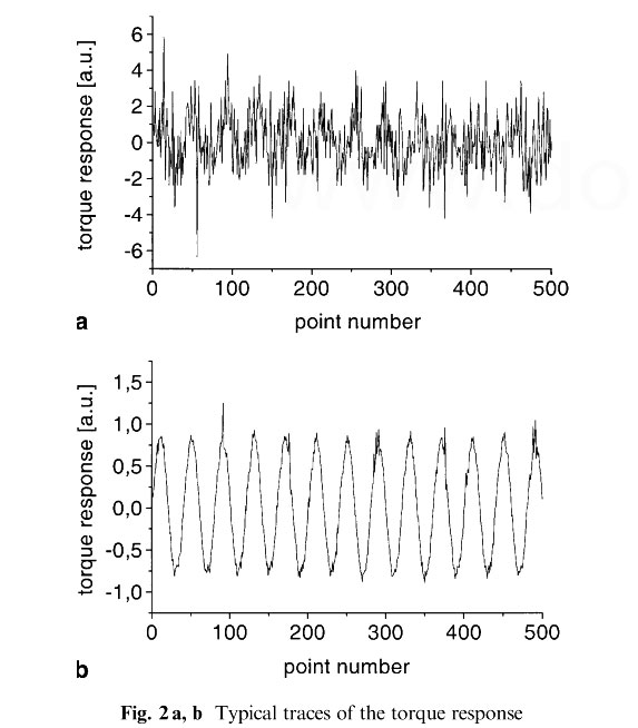
Fig.2a, b Typical traces of the torque response for 0.1 Hz and 0.2% shear amplitude, sampled with 4 Hz sampling rate: a time data taken every 250 ms,no boxcar average, no oversampling; b similar conditions but oversampled with 20 kHz, afterwards boxcar average over 5,000 raw data points. The boxcar average reduces the originally 2.5x 10⁶ raw data points to the displayed 500 data points. Obvious the time data is greatly improved.
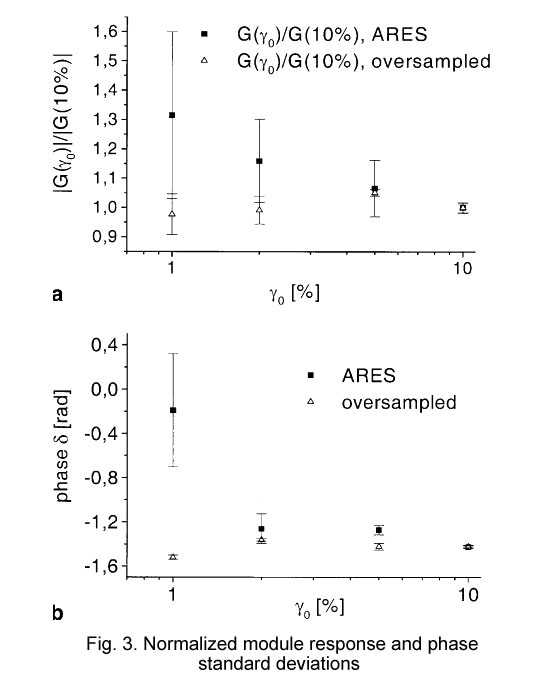
Fig.3 a Normalized module of a 10% polyisobutylene solution where a shear frequency of 0.01 Hz with indicated shear amplitudes was applied. The shear module was normalized to the response at v0= 10% (|G*|≌8.4 Pa). The data observed directly from the ARES is compared with the data observed via the "oversampling" technique. Standard deviations where calculated via several measurements. Sampling rate: 20 kHz, boxcar average over 10,000 points, rheometric data over one cycle, PC data over five cycles. b Phase of a 10% polyisobutylene solution where a shear frequency of 0.01 Hz with different shear amplitudes was applied. The phase lag is displayed as a function of 20. The data observed directly from the A R ES is compared with the data calculated via the "oversampling" technique. Mean values and standard deviations of the phase information where calculated via several measurements.
4 Conclusion
In this article we describe a new data treatment for measuring oscillatory shear response with a significant higher precision than the one originally provided by the manufacturer (Rheometric).
The lower detectable torque limit as supplied by the torque sensor manufacturer has been shown to depend on the magnitude of the random noise, which can be averaged, and not on the magnitude of irreducible systematic errors. Therefore, a very cost-efficient investment can be made, which results in a significant improved precision of rheologically relevant data.
As we have shown experimentally, an improvement by a factor of 3-5 in the minimum torque regime seems to be a realistic estimate if this method were to be implemented by the manufactures.
Acknowledgments It is our great pleasure to thank Prof. H.W. Spiess for continuous support and Dr. P. Reinheimer for early discussions. Financial support within the EU CAPS-project (contract No. FM RX-CT97-00112(DG 12-DLCL)) is gratefully acknowledged by D.v.D. We are also grateful to Dr. N. Willenbacher from the BASF AG Ludwigshafen (Germany) for different Oppanol samples.